
Signal processing
Signals and noise.
The basic purpose of signal processing is to try to retrieve a useful signal from all the background noise and process it so it is meaningful. At radio frequencies there is noise coming from all kinds of sources, mainly from man-made devices such as car ignitions, electrical switching circuits and of course terrestial radio transmissions. Other sources such as lightning can swamp a signal too.
The signals we are looking for are often very difficult to retrieve from the noise and this has been a problem not just for astronomers but ever since telegraph was invented way back in 1837.
In this section I want to introduce some techniques for processing the radio noise in order to extract the desired signal. The following topics are discussed:
Analogue to Digital Conversion
Signal to Noise Ratio
Signal Integration
The Fourier Transform
Analogue to Digital Conversion
Radio signal are continuous waveforms so in order to carry out any computation the waves must be converted into digital format. Some microprocessors have built in analogue to digital convertors and have hardware to process these signals. These are known as DSP series (short for Digital Signal Processor).
If you don't need a DSP but want to take an analogue signal and feed it into a computer for processing, such as a Raspberry Pi, then you can buy devices such as a LabJack which has several Analogue to Digital Conversion (ADC) channels, or you can use a dedicated ADC chip.
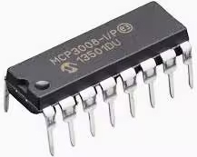
I use the MCP3008 for processing data from my solar flare detector, connected to a Raspberry Pi 4. The MCP3008 is a 10 bit ADC which operates at 200,000 samples per second, adequate for many amateur radio astronomy applications. One of it's useful properties is that it needs no extra components, just a power supply, so it is very simple to connect to a computer. A link to the datasheet can be found in the sidebar.
Signal to Noise Ratio
The Signal to Noise Ratio (SNR) of a system is a very important parameter that gives a measurement of how good the system is at retrieving the signal from the background noise. The most basic expression for SNR is the signal power divided by the noise power. This gives us a simple ratio with no units.
We can write this as SNR = Psignal / Pnoise
However measurements of signal and noise power are more often expressed in decibels. Devices to measure signal levels and noise levels often give their measurements as a ratio of detected value compared with a baseline value, in decibels.
By definition the SNR measured in decibels (referred to as SNRdB) is related to the SNR with no units, by the following expression:
SNRdB = 10 log10(SNR)
Now SNR = Psignal / Pnoise as we saw above.
So we can write SNRdB = 10 log10(Psignal / Pnoise)
Logarithms have transform properties that make them very useful for doing mathematics.
One of the useful transforms is as follows:
Log10(A/B) = Log10(A) - Log10(B), so for example log10(8) - log10(3) = log 10(8/3)
So using this transform, we can write:
10 log10(Psignal / Pnoise) = 10log10(Psignal) - 10log10(Pnoise)
And using the dB conversion above:
SNRdB= PsignaldB - PnoisedB
So to put it another way, the signal to noise ratio (measured in decibels) is equal to the signal level in decibels minus the noise level in decibels. How brilliantly simple!
A worked example:
Suppose we have a device that measures a signal level of 22dB and a noise value of 16dB, the SNRdB would be:
SNRdB= 22dB - 16dB = 6dB
This is the answer in decibels.
If we want to find this as a simple ratio, we can say that SNRdB = 6dB = 10log10(SNR)
Now the definition of a logarithm is that an expression such as X=log10Y means the same as Y=10X
So by the same logic, in this example SNR = 10(6/10) = 100.6=3.981
So the SNR as a simple ratio is 3.981 or in decibels it is 6dB. The signal is nearly 4 times as strong as the noise.
Signal Integration
When attempting to detect galactic hydrogen (see projects), the signal to noise ratio is so small that we can't reliably say that we have definitely acquired a signal from a single sample. We need to use a technique for sampling many times, assuming that the noise is random, to extract the signal from the background noise.
Integrating signals is a technique in which a small bandwidth of radio data that centres around a frequency of interest is repeatedly sampled. The sample will have random noise but possibly a desired and hopefully consistent signal buried within it. Samples are repeatedly taken over time, and sequentially added together. The random noise will eventually cancel itself out, but if there is a signal buried in the data it will emerge as it does not cancel itself out.
Imagine we sampled ten data points and acquired the following values:
56 55 47 64 57 72 65 70 49 55
This data was randomly generated to simulate noise, but then a signal was added. Identifying the signal buried within the noise is impossible from just one set of data.
Suppose we took another ten data points from the same frequency range and acquired the following values:
43 45 62 70 45 72 60 52 44 53
And another ten data points:
55 42 62 37 55 72 59 61 54 56
And another ten data points:
37 62 54 51 58 72 57 57 51 56
If you look carefully, can you see a pattern emerging?
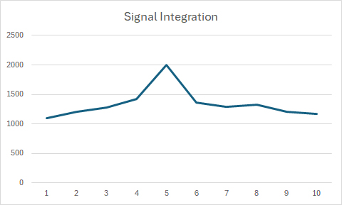
Here is a chart showing what random noise wih a signal embedded in it might look like after just four iterations of the sampled data have been added together:
As mentioned above, signal integration is essential for detecting Galactic hydrogen. It is also necessary for detecting many other radio astronomical sources, for example pulsars.
The Fourier Transform
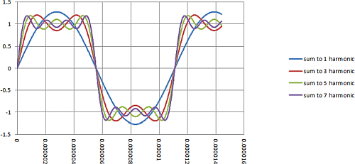
Any introduction to signal processing wouldn't be complete without some discussion of the Fourier Transform. A simple idea but incredibly useful. It takes a waveform in the time domain and uses some not-too-difficult (!) mathematics to convert it into a function in the frequency domain. It hinges on a discovery that every waveform, however random it appears in frequency and/or amplitude, can be broken down into a series of sine waves. A square wave can be shown to be nothing more than lots of sine waves of odd frequency added together:
Planet Analog
This astonishing discovery is fundamental to signal processing. It was made in 1822 by Joseph Fourier, a French mathematician working on a problem regarding heat conduction, and it's application to communications and radio became apparent as the technologies emerged.
What does the Fourier Transform do? It takes a waveform in the time domain, i.e a wave over a period of time, and through a repeated cycle of computations at ever increasing frequencies, it works out how much of each frequency is embedded in the signal.
Suppose we start with a fundamental frequency, say 1Hz. It computes all the possible values that a sine wave would produce at 1Hz and then compares those values with what it actually finds in our wave. It repeats this for 2 Hz, 3Hz and so on. Eventually it will have a series of frequencies which we can imagine along an x axis, and for each frequency it shows the amplitude of our wave at each particular frequency. So the Fourier Transform of a sine wave would be a single spike at that frequency.
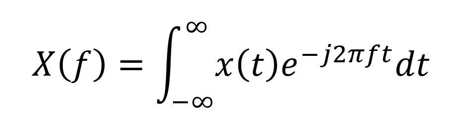
And an explanation of Fouriers triumph wouldn't be complete without the formula itself:
Mathematics Globe
It looks quite daunting. It basically says that the value of a function X of the waveform at frequency f, the X(f) value, on the left hand side, is equal to the value of a function x of the waveform in the time domain at a specific time t, the x(t) component on the right hand side, multiplied by a function e-j2πft at time t. Then repeat for the all values of time from minus infinity to infinity, because a sinewave has no beginning or end.
The function e-j2πft is derived from Euler's formula ejx = cos(x)+jsin(x) where j is the imaginary number, and is equal to √-1. Put simply it is a complex function that gives us the magnitude and phase of a sinusoid of frequency f at time t.
In the side column I have put a link to a really good YouTube video, a very simple explanation of Fourier Transforms using a smoothie recipe, and an explanation of how sine waves combine to make more complex waves.